A Classical Approach to Spike Sorting

Introduction

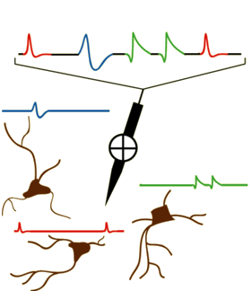
In the field of Neuroscience, one often wants to capture individual neuron activity. This is often done via a microelectrode (or set of microelectrodes) inserted into the brain and recording the time series of voltage readings. Often a times, these readings are extracellular recordings taken within a neighborhood of neurons. The task of taking this time series and extracting the action potential signatures from individual neurons is called spike sorting. A modified diagram from the UCLA PDA Wiki page [1] illustrating the process is shown below.

Approach

Initially, we have a raw time series of extracellular voltage recordings. This is often smoothed out using a bandpass filter. One common preprocessing step is to threshold the neurons and window each detected action potential inferred by the spike threshold crossing points. Finally, the windowed data is projected into a feature space and clustered in order to find the underlying neural signatures of each individual neuron.

A lot of the signal filtering, thresholding, and windowing is generally done using a priori knowledge of the experiment, method of data acquisition, underlying physiology, and general neuroscience knowledge. Sometimes, this may mean a scientist will analyze the neural signal traces visually and manually tune a threshold to detect spikes.

For the sake of brevity, we will focus on the final stage of spike sorting; given the windowed action potentials detected, we want to determine the underlying neurons. One original approach [2] is to use principal component analysis (PCA) in conjunction with K-Means.

Dataset

In order to demonstrate the process of spike sorting, we need a dataset.

The first dataset found contains extracellular recordings from anterior lateral motor cortex neurons in adult mice during experiments [3] [4]. This data is provided courtesy of crcns.org.

In this dataset, multiple (3-8 per subject mouse) electrodes were used in order to sample data from multiple locations. Voltages were recorded at 312.5 kHz with a voltage resolution of 14 bits [4]. This dataset is included to give one an idea of what extracellular recordings look like. Some of the raw voltage traces recorded are shown below.

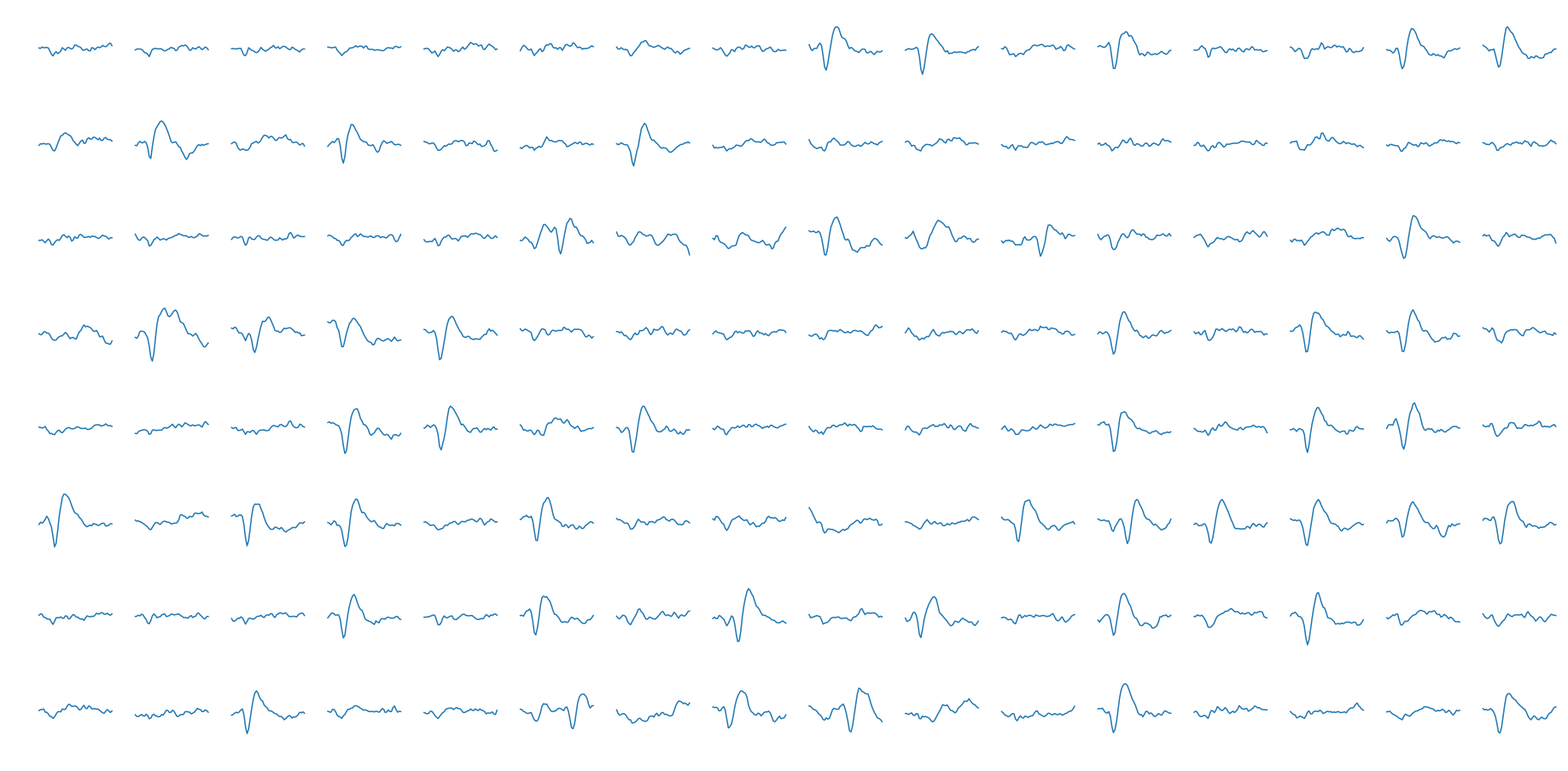
We want to skip the thresholding stage for now, so we will be using a different dataset for the spike sorting. Another dataset provided on crcns.org has pre-segmented extracellular action potentials collected by the Laboratory of Dario Ringach at UCLA. This data was collected from V1 (visual cortex) neurons of macaque monkeys using a 128 channel microelectrode array. At the segmented action potential stage stage, the data is digitized at 8 bits and sampled at 30 kHz. We will use the segmented spike set from the first channel of the first subject. A few individual data samples shown below.

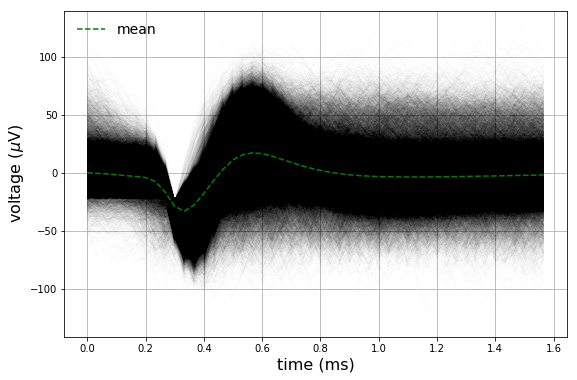
The entire (\(n \approx 90,000\)) dataset in addition to the mean are also plotted.

Spike Sorting

The first step for our spike sorting algorithm will be feature extraction; we will be using principal component analysis to do this. For those unfamiliar with the algorithm, it is recommended to read the Wikipedia page [8] in addition to the relevant references included [9] [10].

The way we will be using it will be treating each windowed action potential as a feature vector in order to compute the principal components. This is an effective approach, since there are distinct covariances for each neural signature. We will be using the eigen-decomposition technique [10].

Given a data matrix \(\mathbf{X}_{t \times n}\), where t is the time index of the sample, and n is the index of each windowed action potential, we want to project into a feature space with \(m\) features per sample; we want to compute the data matrix \(\mathbf{F}_{m \times n}\). Since PCA computes principal components that the original data is projected onto, we can represent PCA as a linear operator \(\mathbf{U}\), where each row represents a principal component.

\[\mathbf{F}_{m \times n} = \mathbf{U}_{m \times t} \mathbf{X}_{t \times n}\]

We will compute the transformation matrix via an eigen-decomposition of the covariance matrix.

First, we de-mean the data:

\[\mathbf{X}_0 = \mathbf{X} - E{[\mathbf{X}]}\]

We then go on to compute the covariance matrix:

\[\mathbf{C} = \mathbf{X_0}\mathbf{X_0}^T\]

Afterwards, we compute an eigendecomposition [6] on the covariance matrix, and sort the eigenvalue-eigenvector \((\mathbf{v}_i, \lambda_i)\) pairs by descending eigenvalue:

\[Eig\{\mathbf{C}\} = \{ ( \lambda_i, \mathbf{v}_i) \mid \lambda_i \geq \lambda_{i-1} \, \forall \lambda_i, \,\, i = 1 ... t \}\]

There is meaning behind each eignenvalue-eigenvector pair: The eigenvector represents the principal component, whereas the eigenvalue represents how much variance is captured by the corresponding principal component. Given the sort by descending eigenvalue, first principal component captures more variance in the data than the second principal component, and so on. The resulting eigenvectors, or principal components, are organized into a matrix:

\[\mathbf{U} = \begin{pmatrix} & \mathbf{v}_1 & \\ & \mathbf{v}_2 & \\ & \vdots & \\ & \mathbf{v}_m & \end{pmatrix}\]

At this stage, we need to choose \(m \leq t\): how many principal components to keep. Now that we have covered how PCA is used in this use case, we will turn our attention to tuning \(m\).

Let’s plot two metrics from our principal component analysis:

• The normalized variance

\[\frac{\lambda_i} {\sum_{k=1}^{t} {\lambda_k}}\]

• The cumulative normalized variance

\[\frac{ \sum_{k=1}^{i} {\lambda_k}} {\sum_{k=1}^{t} {\lambda_k}}\]

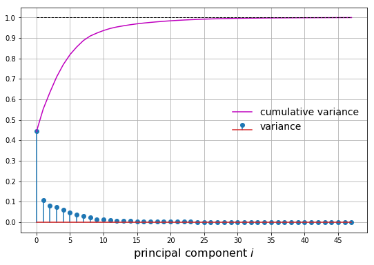
Let’s say we want to capture at least 75% of the variance. We choose \(m\) principal components such that the cumulative normalized variance is greater than 0.75. In this case, we choose \(m=4\). We can then plot the first 4 principal components as well as the projected samples in the feature space:

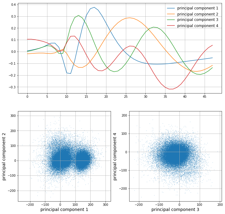
It is clear that the first principal component looks a lot like an action potential. The latter few principal components look less and less like action potentials as their corresponding variance decreases; they are less important. From looking at the scatter plots of the data in the feature space, it is clear that the most predominant clusters arise along the first principal component. However, as we go on to components 2, 3, and 4, it seems like we are capturing more noise than valuable information.

We will now run k-means clustering [7] [15] on the data projected into the feature space, or, more formally, the feature matrix \(\mathbf{F}\). It looks like there are 2 clusters from our previous plots, so we will choose \(k=2\) for k-means.

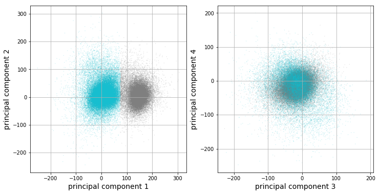
The clustering results corroborate our previous observations: only the first principal component looks like it is capturing valuable information in this dataset. The vertical boundary between the two clusters further implies that only the first component appears to be valuable for our analysis. Let’s get at intuition of what each cluster looks like by analyzing statistics of each cluster’s corresponding data points. For each cluster, there are a set of corresponding windowed action potentials. A plot of clustered means with 95% confidence intervals, in addition to the full dataset mean, are plotted below.

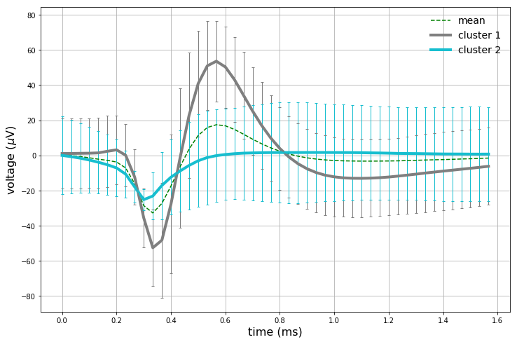
We have now captured (presumably) 2 different neurons. The full dataset mean is also plotted as a sanity check. The first cluster mean captured strongly resembles an action potential, and also strongly corresponds with the full dataset mean. The second cluster does hint at some background neuronal activity, as the initial downwards turn of the curve happens earlier than the first cluster mean. Interestingly enough, the second cluster does not have a pronounced upward spike like the first cluster.

A fundamental question arises here: are we really capturing two neurons, or is the second cluster simply noise or an artifact of our clustering technique? This is a very difficult question to answer, and is often tackled by testing various spike sorting techniques on the data, and using a priori knowledge of the experimental design [2].

We have just gone through one of the most basic forms of spike sorting. In order to get better results, many different tweaks could be applied. Some potential additional steps include:

• More sophisticated pre-threshold filtering
• More sophisticated thresholding
• Rejecting noisy windowed samples
• Rejecting non-spike windowed samples
• More advanced feature extraction
• More intelligent clustering
• Using all channels of the microelectrode array
• Incorporating the electrode geometry and physics into the algorithm
• Many, many more undiscovered improvements

Since the data we used was already in windowed form, it is possible that some of these fine tuning steps up to the windowing stage have already been implemented. Spike detection and classification is a key component in brain-machine interfaces [12] [13]; Many neuroprosthetics [13] [14] operate on extracellular recordings. This is still a very active area of research, and it is likely to further accelerate once commercial neural implants become more widespread.

Note from the Author

I hope you learned just as much reading this post as I did creating it. Questions? Comments? My contact information is available here.

Citation

Please cite this post using the BibTex entry below.

@misc{
author = {Liapis, Yannis},
title = {A Classical Approach to Spike Sorting},
journal = {},
type = {Blog},
number = {December 29},
year = {2017},
howpublished = {\url{http://yliapis.github.io}}

This work is licensed under a Creative Commons Attribution 4.0 International License.

References

[1] “Neural Spike Sorting”, PDA Group Wiki (UCLA)

[2] Quiroga, R. Q., “Spike Sorting”, Scholarpedia 2.12 (2007): 3583. Web. 14 Feb. 2016

[3] N. Li et al, “A motor cortex circuit for motor planning and movement”, Nature 519, 51–56 (05 March 2015), doi: 10.1038/nature14178

[4] N. Li et al, “Extracellular recordings from anterior lateral motor cortex (ALM) neurons of adult mice performing a tactile decision behavior”, CRCNS.org (2014), http://dx.doi.org/10.6080/K0MS3QNT

[5] I. Nauhaus, D. L. Ringach, “Precise Alignment of Micromachined Electrode Arrays With V1 Functional Maps”

[6] “Eigendecomposition of a matrix”, Wikipedia

[7] J. A. Hartigan et al, “Algorithm AS 136: A K-Means Clustering Algorithm”. Journal of the Royal Statistical Society, Series C 28 (1979)

[8] “Principal component analysis”, Wikipedia

[9] S. Wold et al, “Principal component analysis”, Chemometrics and Intelligent Laboratory Systems, Vol 2 Iss 1-3, Aug 1987, pp 37-52

[10] H. Abdi, L. J. Williams, “Principal component analysis”, WIREs Computational Statistics

[11] M. S. Lewicki. “A review of methods for spike sorting: the detection and classification of neural action potentials,” Comput. Neural Syst. 9, R53- R78, (1998)

[12] D. R. Kipke et al, “Silicon-substrate intracortical microelectrode arrays for long-term recording of neuronal spike activity in cerebral cortex”, IEEE Transactions on Neural Systems and Rehabilitation Engineering, Vol 11, Iss 2, June 2003

[13] D. Borton et al “Personalized Neuroprosthetics”, Science Translational Medicine 06 Nov 2013: Vol. 5, Issue 210, pp. 210rv2, DOI: 10.1126/scitranslmed.3005968

[14] J. J. Shih et al, “Brain-Computer Interfaces in Medicine”, Mayo Clin Proc. 2012 Mar; 87(3): 268–279, doi: 10.1016/j.mayocp.2011.12.008

[15] “k-means clustering”, Wikipedia