The Kalman Filter

Introduction

This post is dedicated to one of the most understated techniques in science and engineering: the Kalman Filter. This filter is used in numerous technologies, such as GPS, autonomous vehicle control, missile guidance, robotic motion planning, and financial signal processing. In addition to all of the technologies not mentioned, this list will keep growing in the future.

So, what does this filter do?

The Kalman Filter makes an educated guess about the state of a dynamical system given incomplete and/or noisy information.

Background - The Bayes Filter

To begin, let’s introduce the concept the Kalman Filter is based upon: Recursive Bayesian estimation, or the Bayes filter. Simply put, the goal is to estimate an unknown probability density function recursively over time using incomplete or noisy measurements [4].

We can represent our dynamical system as a hidden markov model (HMM).

\(\mathbf{x}_k\) represents the state of the dynamical system at timestep \(k\), and \(\mathbf{z}_k\) represents the measurements at timestep \(k\).

We want to estimate the current state, or a distribution over the current state, given a sequence of measurements up to the present time.

\[p(\mathbf{x}_k|\mathbf{z}_k, \mathbf{z}_{k-1}, ..., \mathbf{z}_1)\]

In the equation’s current form, things look a bit uncertain on how to proceed. Given the markov assumption, and the HMM structure of our model, we can break things down further.

\[p(\mathbf{x}_k|\mathbf{x}_k, \mathbf{x}_{k-1}, ..., \mathbf{x}_{0}) = p(\mathbf{x}_k|\mathbf{x}_{k-1})\] \[p(\mathbf{z}_{k}|\mathbf{x}_k, \mathbf{x}_{k-1}, ..., \mathbf{x}_{0}) = p(\mathbf{z}_{k}|\mathbf{x}_k)\]

The joint distribution can thus be computed as follows:

\[p(\mathbf{x}_k, \mathbf{x}_{k-1}, ..., \mathbf{x}_0, \mathbf{z}_k, \mathbf{z}_{k-1}, ..., \mathbf{z}_1) = p(\mathbf{x}_0)\prod^{k}_{i=1}{p(\mathbf{z}_{i}|\mathbf{x}_i) p(\mathbf{x}_i|\mathbf{x}_{i-1})}\]

This is all fairly straight forwards so far given our model. How do we make any sense of all this in order to get our state estimate, given we only observe \(\mathbf{z}\)?

There are two steps to the bayes filter: Pedict, and Update

Prediction

We can formulate the prediction step as follows:

\[p(\mathbf{x}_k | \mathbf{z}_{1:k-1}) = \int{ p(\mathbf{x}_k | \mathbf{x}_{k-1}) p(\mathbf{x}_{k-1} | \mathbf{z}_{1:k-1})d\mathbf{x}_{k-1} }\]

Looking at this formulation more closely, there is a clear pattern. The second term in the integral is simply the previous timestep’s predict step! This is where we can finally implement the recursive structure of the filter, which greatly simplifies things.

Going back one step:

\[p(\mathbf{x}_k | \mathbf{z}_{1:k-1}) = \int{ p(\mathbf{x}_k | \mathbf{x}_{k-1}) \left(\int{ p(\mathbf{x}_{k-1} | \mathbf{x}_{k-2}) p(\mathbf{x}_{k-2} | \mathbf{z}_{1:k-2}) d\mathbf{x}_{k-2} }\right) d\mathbf{x}_{k-1} }\]

Going back all the way:

\[p(\mathbf{x}_k | \mathbf{z}_{1:k-1}) = \int{ p(\mathbf{x}_k | \mathbf{x}_{k-1}) \left(\int{ p(\mathbf{x}_{k-1} | \mathbf{x}_{k-2}) ... \left(\int{ p(\mathbf{x}_{1} | \mathbf{x}_{0}) p(\mathbf{x}_{0}) d\mathbf{x}_{0} }\right) ... d\mathbf{x}_{k-2} }\right) d\mathbf{x}_{k-1} }\]

Updating

So, now that we have the prediction, we want to update given our current measurement \(\mathbf{z}_k\). We’ll simply use Baye’s rule here.

\[p(\mathbf{x}_k | \mathbf{z}_{1:k-1}) = \frac{p(\mathbf{z}_{k}|\mathbf{x}_k) p(\mathbf{x}_k | \mathbf{z}_{1:k-1})} {p(\mathbf{z}_k | \mathbf{z}_{1:k-1})}\]

The denominator can be rewritten as follows:

\[p(\mathbf{z}_k | \mathbf{z}_{1:k-1}) = \int{ p(\mathbf{z}_k | \mathbf{x}_{k}) p(\mathbf{x}_k | \mathbf{z}_{1:k-1}) d\mathbf{x}_k}\]

This looks very similar to the numerator. In fact, it is simply the integral of the numerator over the current step! This is just a normalizing term, and is constant relative to \(\mathbf{x}\).

\[p(\mathbf{z}_k | \mathbf{z}_{1:k-1}) = \alpha\]

This term can simply be ignored in application of the filter.

\[p(\mathbf{x}_k | \mathbf{z}_{1:k-1}) \propto p(\mathbf{z}_{k}|\mathbf{x}_k) p(\mathbf{x}_k | \mathbf{z}_{1:k-1})\]

Summary

We now have the two key components of a Bayesian filter:

Predict

\[p(\mathbf{x}_k | \mathbf{z}_{1:k-1}) \leftarrow \int{ p(\mathbf{x}_k | \mathbf{x}_{k-1}) p(\mathbf{x}_{k-1} | \mathbf{z}_{1:k-1}) d\mathbf{x}_{k-1} }\]

Update

\[p(\mathbf{x}_k | \mathbf{z}_{1:k-1}) \leftarrow p(\mathbf{z}_{k}|\mathbf{x}_k) p(\mathbf{x}_k | \mathbf{z}_{1:k-1})\]

The Kalman Filter

The Kalman Filter is one of the most basic implementation of a Bayesian Filters: the distributions of the variables will be continuous and Gaussian distributed. In this case, we simply need to keep track of the mean and covariance of the state we are tracking.

Notation

• \(\mathbf{F}_k\), the state transition model
• \(\mathbf{H}_k\), the observation model

• \(\mathbf{B}_k\), the control input model (when needed)

• \(\mathbf{K}_k\), the Kalman gain (more on this later)

Since we are assuming the probabilities tracked are Gaussian, we simply need to track means and covariances:

• \(\mathbf{x}_k\), the state

• \(\mathbf{Q}_k\), the covariance of the state transition noise

• \(\mathbf{z}_k\), the measurement
• \(\mathbf{R}_k\), the covariance of the observation noise

Models

Our state transition model is written as follows:

\[\mathbf{x}_k = \mathbf{F}_k\mathbf{x}_{k-1} + \mathbf{B}_k\mathbf{u}_k + \mathbf{w}_{k}\]

Where \(\mathbf{w}_{k} \sim \mathcal{N}(\mathbf{0}, \mathbf{Q}_k)\) represents our state transition noise. Our measurement model is written as follows:

\[\mathbf{z}_k = \mathbf{H}_k\mathbf{x}_k + \mathbf{v}_k\]

Where \(\mathbf{v}_{k} \sim \mathcal{N}(\mathbf{0}, \mathbf{R}_k)\) represents our state transition noise.

Given these conditions, we want to tract the following quantities:

• \(\mathbf{\hat{x}}_k\), the state estimate
• \(\mathbf{P}_k\), the state estimate error covariance

From these models, we can relate things back to the Bayesian filter:

\[p(\mathbf{x}_k | \mathbf{x}_{k-1}) = \mathcal{N}(\mathbf{F}_k\mathbf{x}_{k-1} + \mathbf{B}_k\mathbf{u}_k, \mathbf{Q}_k)\] \[p(\mathbf{z}_k | \mathbf{x}_{k}) = \mathcal{N}(\mathbf{H}_k\mathbf{x}_k, \mathbf{R}_k)\] \[p(\mathbf{x}_k | \mathbf{z}_{1:k}) = \mathcal{N}(\mathbf{x}_k, \mathbf{P}_k)\]

Given this model, we can derive the predict and update steps. The predict step is given. The update step, however, has a crucial component that must be derived: the Kalman gain \(\mathbf{K}_k\).

Predict

$$ \mathbf{\hat{x}}_{k \mid k-1} = \mathbf{F}_k\mathbf{\hat{x}}_{k-1 \mid k-1} + \mathbf{B}_k\mathbf{u}_k $$	Predicted state estimate
$$ \mathbf{P}_{k \mid k-1} = \mathbf{F}_k\mathbf{P}_{k-1 \mid k-1}\mathbf{F}_k^\mathrm{T} + \mathbf{Q}_k $$	Predicted estimate covariance

Update

$$ \tilde{\mathbf{y}}_k = \mathbf{z}_k - \mathbf{H}_k\hat{\mathbf{x}}_{k\mid k-1} $$	pre-fit residual
$$ \mathbf{S}_k = \mathbf{R}_k + \mathbf{H}_k \mathbf{P}_{k\mid k-1} \mathbf{H}_k^\mathrm{T} $$	pre-fit residual covariance
$$ \mathbf{K}_k = \mathbf{P}_{k\mid k-1}\mathbf{H}_k^\mathrm{T} \mathbf{S}_k^{-1} $$	Optimal Kalman gain
$$ \hat{\mathbf{x}}_{k\mid k} = \hat{\mathbf{x}}_{k\mid k-1} + \mathbf{K}_k\tilde{\mathbf{y}}_k $$	Updated state estimate
$$ \mathbf{P}_{k|k} = (\mathbf{I} - \mathbf{K}_k \mathbf{H}_k )\mathbf{P}_{k|k-1}(\mathbf{I} - \mathbf{K}_k \mathbf{H}_k )^{\mathrm{T}}+\mathbf{K}_k\mathbf{R}_k\mathbf{K}^{\mathrm{T}}_k $$	Updated estimate covariance

The full derivation is beyond the scope of this post, although those interested in learning more are recommended references [1], [5], and [6]. In summary, the Kalman filter minimizes the square error between the true state and estimated state,

\[E[ \| \mathbf{x}_{k} - \hat{\mathbf{x}}_{k} \| ]\]

There are many different formulations of the Kalman filter, and we have covered the most basic formulation.

Experiments

To illustrate the concept of the Kalman Filter, we will construct a toy example: Given a particle’s 1 dimentional position over time, we will try to estimate its velocity.

Notation

• \(x\) : position
• \(v\) : velocity
• \({\Delta}t\) : timestep

Given these quantities, we can now formulate our problem. Kalman filters are not plug and play like many other signal processing and machine learning techniques; They need to be tailored and fine tuned to the problem at hand.

\(\mathbf{z} = \begin{pmatrix} x \end{pmatrix}\) (measurement)

\(\mathbf{x} = \begin{pmatrix} x \\ v \\ \end{pmatrix}\) (state)

\(\mathbf{H} = \begin{pmatrix} 1 \\ 0 \\ \end{pmatrix}\) (measurement process)

\(\mathbf{F} = \begin{pmatrix} 1 & {\Delta}t \\ 0 & 1 \\ \end{pmatrix}\) (state transition)

Now that we have formulated our problem, we generate some synthetic measurement data.

\[\mathbf{z}_k = \mathbf{f}(k\Delta{t}) + \mathbf{\nu_k}, \quad \mathbf{\nu}_k \sim \mathcal{N}(\mathbf{0}, \mathbf{R})\]

We have chosen our true position to be modeled by the sigmoid [7] function ( $ \mathbf{f}() $ ) over time.

)

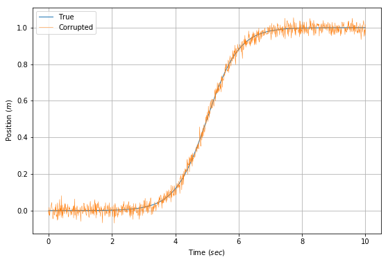
Given this data, we can compute the velocity as \(\Delta{x}/\Delta{t}\). However, the corrupting noise causes some very serious issues that completely destroy our estimate. The corrupting influence of the noise multiplies when trying to estimate velocity in the graph below.

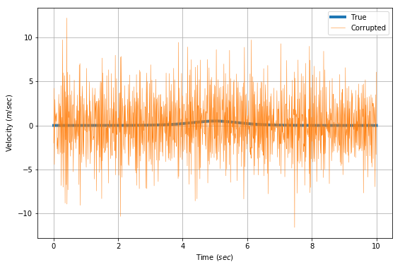
This is why we use a Kalman filter. The model calculation is severely corrupted by the noise.

In order to implement our Kalman filter, we need to estimate two quantities a priori: the observation covariance $\mathbf{R}$ and the state transition covariance $\mathbf{Q}$.

Given we generated the noise, the observation covariance is already known. While it may seem like there is no state transition covariance in this model, this couldn’t be further from the truth; there is a hidden control input, acceleration.

\[\mathbf{x}_k = \mathbf{F}\mathbf{x}_{k-1} + \mathbf{G}a_k\]

Where $ \mathbf{G} $ is the effect of acceleration on our state. Written explicitly,

\[\begin{pmatrix} x_k \\ v_k \\ \end{pmatrix} = \begin{pmatrix} 1 & \Delta{t} \\ 0 & 1\\ \end{pmatrix}\begin{pmatrix} x_{k-1} \\ v_{k-1} \\ \end{pmatrix} + \begin{pmatrix} \frac{\Delta{t}^2}{2} \\ \Delta{t} \\ \end{pmatrix}a_k\]

Thus, $ \mathbf{Q} $ can be estimated as

\[\mathbf{Q} = \mathbf{G}\mathbf{G}^\mathrm{T}\sigma_a^2\]

\(\sigma_a\) is another free parameter that can be estimated by the expected variance of the acceleration. For the sake of argument, the variance is calculated from the original acceleration data as $ Var[\frac{\Delta^2{x}}{\Delta{t}^2}] $. The graphs below show the application of a Kalman filter to estimate velocity in our problem stated. A moving average on the direct calculation of velocity is shown as a comparison.

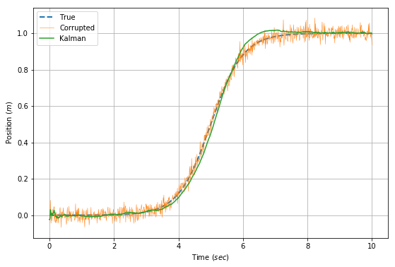
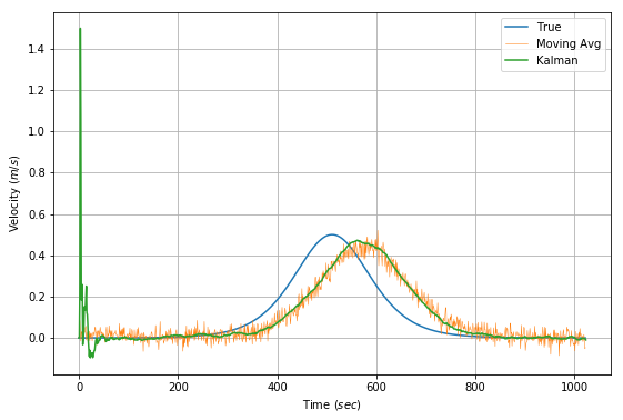
It is clear that the Kalman filter performs much better than a moving average at filtering out the noise. The spike at the beginning of the velocity estimation is due to the beginning period where the filter has seen few samples, is more susceptible to the corrupting influence of noise. The delay of the filter is inevitable, since a number of samples need to be read to register a change. A more responsive filter would be more noisy.

Note from the Author

I hope you learned just as much reading this post as I did creating it. Questions? Comments? My contact information is available here.

Citation

Please cite this post using the BibTex entry below.

@misc{
author = {Liapis, Yannis},
title = {The Kalman Filter (draft)},
journal = {},
type = {Blog},
number = {Nov 10},
year = {2018},
howpublished = {\url{http://yliapis.github.io}}

This work is licensed under a Creative Commons Attribution 4.0 International License.

References

[1] R. Faragher, “Understanding the Basis of the Kalman Filter Via a Simple and Intuitive Derivation”, IEEE Signal Processing Magazine, September 2012, pp 132

[2] R. E. Kalman, “A New Approach to Linear Filtering and Prediction Problems”, Transactions of the ASME–Journal of Basic Engineering, 1960, 82 (Series D): 35-45

[3] T. Babb, “How a Kalman filter works, in pictures”, Bzarg, 2015

[4] “Recursive Bayesian estimation”, Wikipedia

[5] N. Shimkin, “Derivations of the Discrete-Time Kalman Filter”, Israel Institute of Technology, 2009

[6] V. Yadav, “Kalman filter: Intuition and discrete case derivation”, Towards Data Science, 2017

[7] “Sigmoid function”, Wikipedia