Non Negative Matrix Factorization
Introduction
The purpose of this post is to give a simple explanation of a powerful feature extraction technique, non-negative matrix factorization.
Non-negative matrix factorization (NNMF, or NMF) is a method for factorizing a matrix into two lower rank matrices with strictly non-negative elements.
Given matrix \(\mathbf{X}\), find \(\mathbf{W}\) and \(\mathbf{V}\) such that
\[\mathbf{X}_{m \times n} \approx \mathbf{W}_{m \times d}\mathbf{V}_{d \times n}\]Where all elements of \(\mathbf{X}\), \(\mathbf{W}\), and \(\mathbf{V}\) are strictly nonnegative.
Intuition
Why would we want to do this? Let’s assume \(X_{m \times n}\) represents a data matrix of \(n\) samples with \(m\) features. We want to capture the underlying structure of the data. There are many different ways to look at this algorithm.
Let’s take into account the amount of elements:
\[n_1 = |\mathbf{X}| = mn\] \[n_2 = |\mathbf{W}| + |\mathbf{V}| = md +dn\]In the majority of practical cases, the following inequality holds:
\[n_2 \ll n_1\]Through some math, this implies \(d\) is chosen as follows.
\[d \ll (1/n + 1/m)^{-1}\]Generally, \(d \ll \min(m,n)\) is chosen. The inequality between \(n_1\) and \(n_2\) implies a very fundamental aspect of NMF; we are compressing the data matrix \(\mathbf{X}\). While we try to find an accurate representation of \(\mathbf{X}\) as a product of \(\mathbf{W}\) and \(\mathbf{V}\), the two factorized matrices capture information about the underlying structure of the data.
Given \(m\) instances of \(n\) features, \(\mathbf{W}\) can be interpreted as a feature matrix, whereas \(\mathbf{V}\) can be interpreted as the coefficients matrix. In other words, each row of \(\mathbf{W}\) represents an additive basis, whereas each column of \(\mathbf{V}\) represents the basis weighting for each sample reconstruction.
Due to the non-negativity constraint, the features are strictly additive. This property results in sparse feature representations [1], as well as one of NMF’s core strengths: It automatically clusters the data. Unlike PCA which simply rotates the covariance matrix, NMF builds a sparse-basis representation of the data.
One original application of this algorithm was to detect additive objects in images [1]. An excerpted image from the paper is shown below.
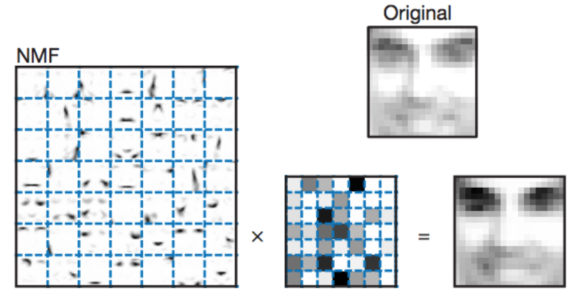
It is immediately apparent that the leftmost matrix of images is capturing facial features. Common patterns such as eyebrows, eye shadows, lips, and facial outlines are being detected and stored by the algorithm with no context other than a set of facial images. These facial features form the sparse additive basis with which faces can be reconstructed.
Algorithm
Unfortunately, this is a non-convex optimization problem [2]. There are multiple different solutions given there is not one, but two matrices to optimize. Different constrains are often added to narrow the solution space. This is a very deep problem, so for the sake of argument, we will take a look at one of the techniques proposed by Lee & Seung [2]: let’s minimize the \(L_2\) norm of the residuals between the original and reconstructed dataset (essentially the squared error).
\[\operatorname*{arg\,min}_{\mathbf{W},\mathbf{V}} {\|}{\mathbf{X} - \mathbf{W} \mathbf{V}}{\|}_2\]We will use the multiplicative update rule proposed [2]. Below are the two update rules.
\[\mathbf{W} \leftarrow \mathbf{W} \odot \frac{\mathbf{X} \mathbf{V}^T}{\mathbf{W} \mathbf{V} \mathbf{V}^T}\] \[\mathbf{V} \leftarrow \mathbf{V} \odot \frac{\mathbf{W}^T \mathbf{X}}{\mathbf{W}^T \mathbf{W} \mathbf{V}}\]The optimization process applies these updates in succession at each training iteration. The proof is beyond the scope of this post; a more thorough explanation is available in the source paper [2]. The gist of this rule is that under certain assumptions, the \(L_2\) norm of the residuals never increases under these updates. This approach is different from the traditional use of gradient decent, which uses an additive update scaled by a learning rate, rather than a multiplicative update.
Note that there are many different ways to solve this problem, and most packages use highly optimized algorithms that will generally produce better results than the plain algorithm shown above. Nonetheless, we will stick with the basic update rules shown above for our experiments. For a more rigorous review of various algorithms, the reader is directed to N. Gillis’s papers [8] [9].
Experiments
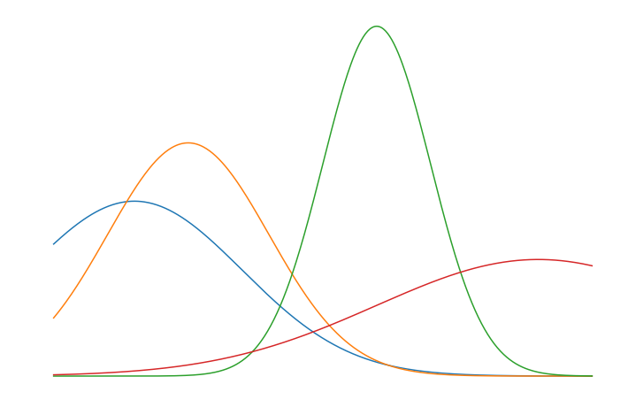
Since this is an unsupervised learning algorithm, let’s try to reverse engineer an additive mixture of gaussians with fixed means, fixed variances, but stochastic amplitudes. Gaussian basis vectors were chosen to make visualization simpler; almost any arbitrary nonnegative basis set could have been used. Each sample is a vector.
\[\mathbf{x}_{i} = \displaystyle\sum_{k=1}^{d} \nu_{i,k} \mathbf{g}_{k}, \quad \nu_{i,k} \sim U(0,1)\] \[\mathbf{g}_{k} = f( \mathbf{t} | \mu_k, \sigma_k)\]\(\mathbf{g}_{k}\) represents a gaussian, where \(f\) is the well known probability density function of a gaussian, and \(\mathbf{t}\) represents the input vector to the pdf. Let’s generate \(d = 4\) basis vectors with 512 samples each. Below are the basis vectors chosen.
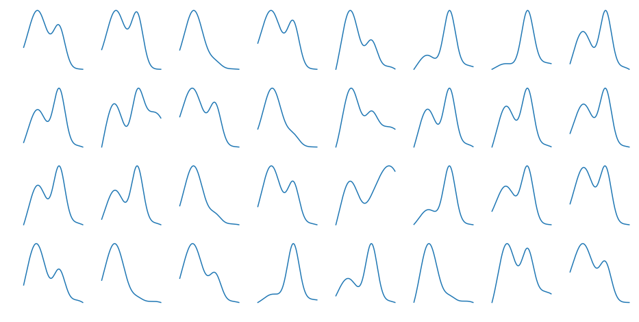
A total of ~16k samples were generated. A few \(\mathbf{x}_i\) samples generated are shown below.
We run the algorithm for 256 steps and log the loss and learned basis vectors during training. The two graphs below show the static \(\mathbf{g}_k\) vectors and the evolving \(\mathbf{W}_{:,k}\) vectors on the left, and the loss (Mean Squared Error) curves on the right.
Over time, \(\mathbf{W}\) evolves from white noise to smooth curves closely matching the \(\mathbf{g}_k\) vectors. From more careful observation of the animation, a few observations are apparent. The first few iterations remove a lot of noise present. As the majority of the noise is removed, the approximated basis vectors begin to shift to resemble the initial basis vectors. This is where the clustering property of NMF becomes clearer; each vector is an underlying source of variation in the data. Towards the later iterations, the remaining amount of noise and mismatch between the curves is slowly taken away.
Below we can see some examples of samples and their reconstructions changing over time.
This is just a toy example of one way the algorithm can be used. Common applications include genomics/bioinformatics [4], text mining [5], image processing [2], and time series (often blind source separation) [6] [7].
Note from the Author
I hope you learned just as much reading this post as I did creating it. Questions? Comments? My contact information is available here.
Citation
Please cite this post using the BibTex entry below.
@misc{
author = {Liapis, Yannis},
title = {Non Negative Matrix Factorization},
journal = {},
type = {Blog},
number = {December 6},
year = {2017},
howpublished = {\url{http://yliapis.github.io}}

This work is licensed under a Creative Commons Attribution 4.0 International License.
References
[1] Lee, D. D. & Seung, H. S., “Learning the parts of objects by non-negative matrix factorization”
[2] Lee, D. D. & Seung, H. S., “Algorithms for Non-negative Matrix Factorization”
[3] Langville, N. L. et al, “Initializations for the Nonnegative Matrix Factorization”
[4] Gao, Y. & Church, G., “Improving molecular cancer class discovery through sparse non-negative matrix factorization”
[5] Xu, W. et al, “Document Clustering Based On Non-negative Matrix Factorization”
[6] Schmidt, M. N. & Olsson, R. K.,”Single-Channel Speech Separation using Sparse Non-Negative Matrix Factorization”
[7] Cichocki, A., “New Algorithms for Non-Negative Matrix Factorization in Applications to Blind Source Separation”
[8] N. Gillis, “The Why and How of Nonnegative Matrix Factorization”
[9] N. Gillis, “Introduction to Nonnegative Matrix Factorization”